Industrial Worksurface Documentation
Welcome to the Industrial Worksurface product documentation.
Features
Simulation in the Industrial Worksurface
Simulation in the Industrial Worksurface
Welcome to the Simulation in the Industrial Worksurface documentation. This documentation covers all aspects of the simulation platform.
Documentation Sections
| Section | Description |
|---|---|
| Always-On Model | Learn about the always-on simulation model |
| Simulation Dashboard | Overview of the main simulation dashboard |
| What-If | Running what-if scenarios |
| Integration with Kognitwin | How simulation integrates with Kognitwin |
| Trending | Working with trend data |
| Unit Profiles | Managing unit profiles |
| Download Simulation Files | Downloading simulation project files |
| Admin Portal | Administration portal guide |
Always-On Model
The Always-On Model represents the physical asset as close as possible. It consumes time-series data through the common Kognitwin Time-Series Endpoint to define boundary conditions (e.g. Battery Limits of the simulated process scope, Valve Positions, Controller Setpoints etc.).
The Always On model provides virtual sensors, realtime plant insights and generates snapshots, that can be used for What-If, Re-Play and Look-Ahead simulations.

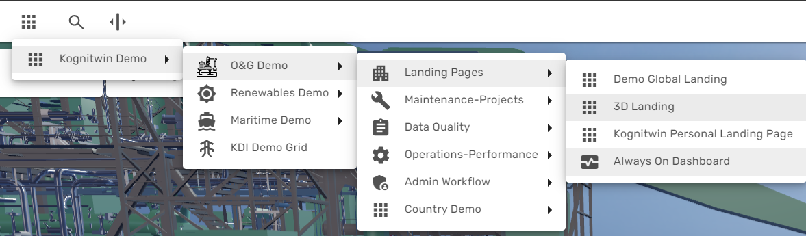
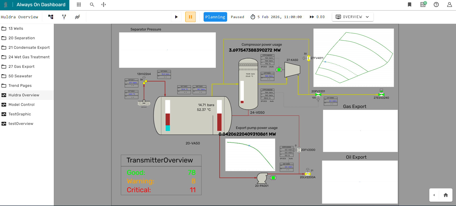
An overview for the main Always-On model instance is provided through the simulation dashboard. It is available from the main menu, typically called "Always On Dashboard":
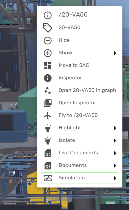
If the simulation workflow is enabled in your environment, you can at any point open the right-click context menu for a specific object or tag (for example from 3D or from a P&ID) and fly to the corresponding tag in the Always-On Dashboard:
Simulation Dashboard Overview
The Simulation dashboard is the main visualization component for integrated Simulations. It contains a rich set of functionality.
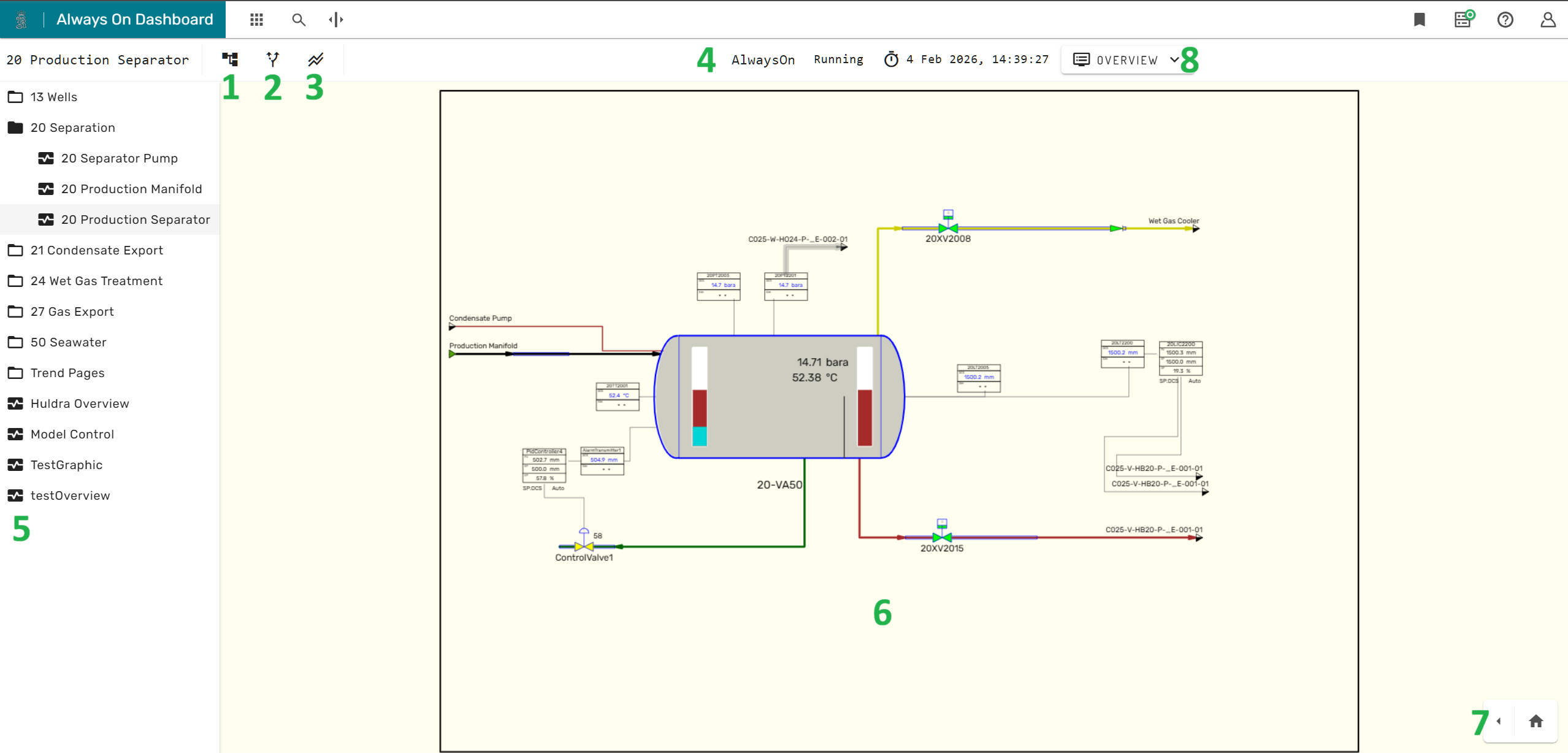
The tree structure icon 1 in the main menu bar shows or hides the process graphic navigation menu 5 on the left side of the screen.
The branching arrows icon 2 opens the What-If Simulation Panel.
The two parallel trend lines icon 3 opens the buffered trends menu.
In the central area of the main menu bar 4 provides status information about the simulation, as for example the running state, the current model time.
In the center of the simulation dashboard, the currently selected simulation graphic 6 is displayed.
In the lower right corner 7, the layer menu and the Unit Profiles can be expanded.
To the right of the main menu bar 8, the module overview menus can be accessed.
Simulation Graphics
Simulation graphics are generated in dedicated desktop software and can be uploaded to Kognitwin through the admin portal.
Simulation graphics can contain the following elements: - A frame with a background - Static text and dynamically updating text fields - Equipment symbols, representing physical or virtual equipment like pumps, valves, compressors and sensors - Connection lines, represent one of the following: - Pipes carrying process fluid (colored lines, color indicates the fluid type) - Cables conducting electricity (black lines) - Mechanical shafts, conveying kinetic energy (black lines) - Low-Voltage Cables conducting signals, e.g. measurement values or control signals (dashed black lines) - Logical states as ON/OFF, TRUE/FALSE (black lines that turn red/green based on the signal)
Equipment symbols provide both left-click interaction (open the module faceplate) and right-click interaction (open the Kognitwin context-menu). Many equipment symbols will also change their appearance based on the state of the equipment they are representing. Valves will for example be green in open position, grey in closed position and yellow in a partially open position.
Connection lines provide left-click interaction (open the stream dialog).
Navigating Simulation Graphics
The simulation dashboard provides the following ways to navigate between simulation graphics:
- The Simulation Graphic Navigator menu
- Stream Connectors
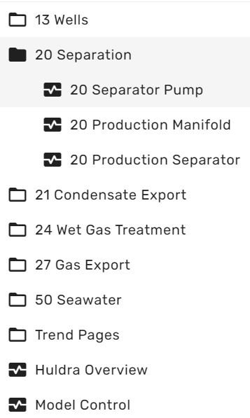
The Simulation Graphic Navigator can be expanded on the left side of the screen as described in the overview section. The simulation graphic navigator uses a tree like structure, branches can be expanded and deflated by clicking on the folder icon. The actual simulation graphics are represented by a small rectangle with a wave function plot. Left-clicking on a graphic icon will open the graphic in the main area of the simulation dashboard.
If connection lines connect signals or process fluid streams across multiple graphics, the two corresponding ends are connected through so called "stream connectors", which typically look like small triangles (arrow tips).
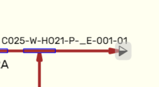
By left-clicking on a stream connector the connecting simulation graphic is opened in the main area of the simulation dashboard.
Module Faceplate
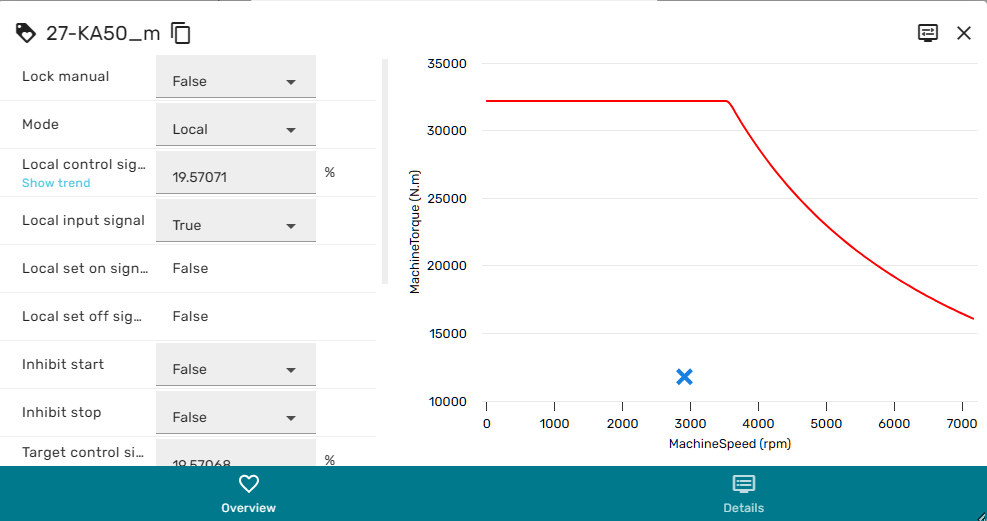
Equipment Symbols (e.g. pumps, transmitters, valves etc.) have dedicated, module specific faceplates.
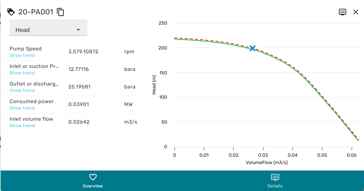 Facplates are generally build up from two main areas, the left area containing the most important variables and their current value, and the right area, that can depict a relevant trend or performance map for the specific equipment.
Some module faceplates also contain a drop-down menu at the top, which allows swapping out the plot or performance map in the right area.
The blue hyperlinks below the variables in the left area allow bringing up a trend for the corresponding variable. Sometimes, variables can have complex data-types that cannot be displayed as a number or text. In these cases, the variable value will become a hyper-link which opens a variable viewer on left-click.
Module Explorer
The Module explorer can be accessed in the following ways:
- From the icon in the upper right corner of module faceplates
- From the right click context menu
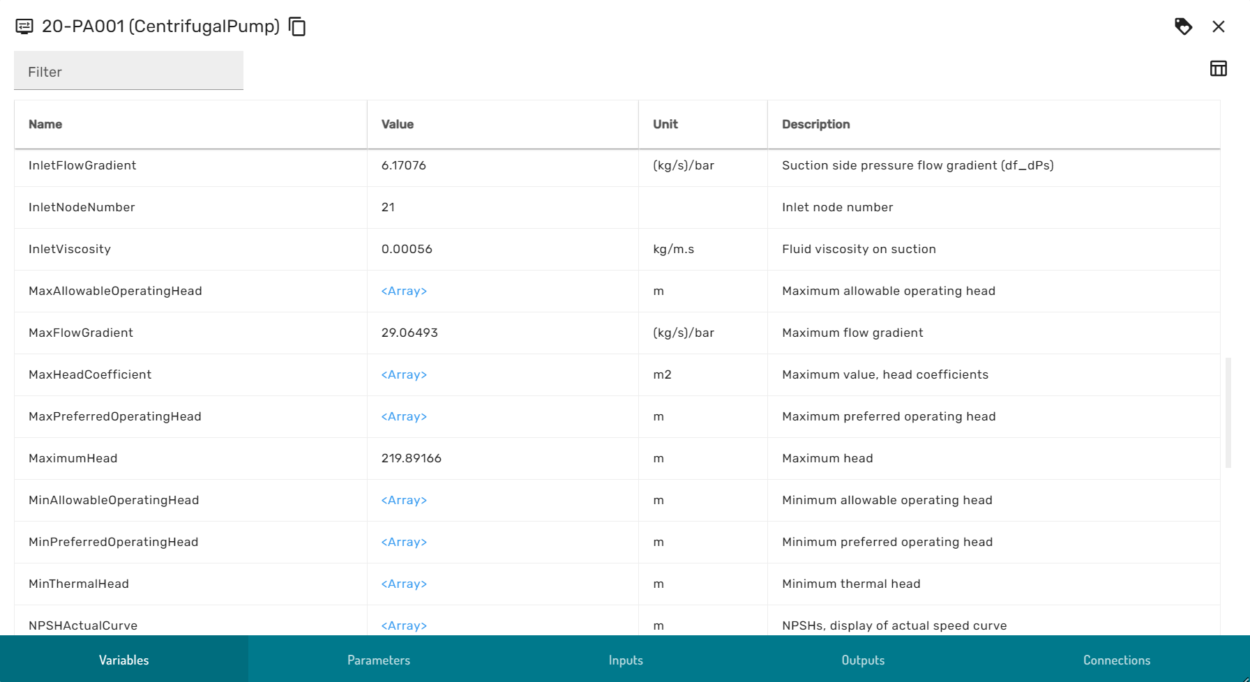
The module explorer is comprised of the following views, that can be swapped through the ribbon menu at the bottom of the dialog:
- Variables: Contains variables that are used internally by the simulator
- Parameters: Contains variables that define the physical and logical properties of equipment, for example design parameters or signal behavior rules
- Inputs: The variables that serve as the input to every simulation calculation step, for example process streams, boundary conditions and signal inputs
- Outputs: The variables that are calculated at every simulation calculation step, the results of the simulation.
- Browse Connections, further described in the browse connection dialog section
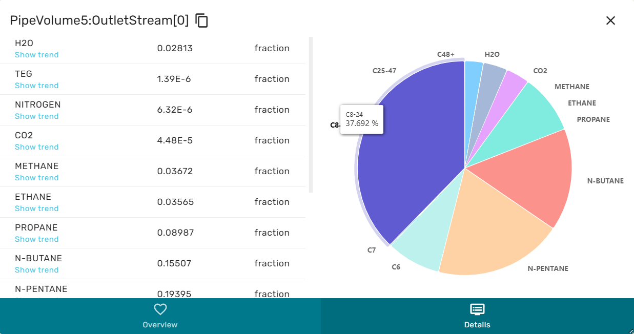
Stream Dialog
The Stream dialog is comprised of a left and a right area, and has an overview and a details view.
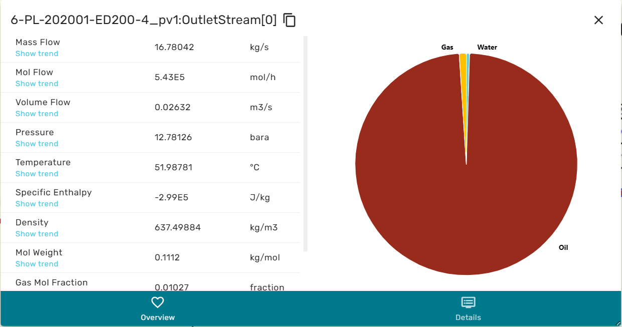
When in overview, the he left area contains a selection of the intensive and extensive thermodynamic properties of the stream, as for example massflowrate, temperature, enthalpy etc. The right area contains a cake diagram of the fluid phases (e.g. oil, gas water). By hovering the mouse over the cake diagram the numerical values for the phase fractions are displayed.
When in Details view, the left area shows a list of all chemical species that are contained in the stream and their concentrations. The right area then shows a cake diagram of the chemical composition. By hovering the mouse over the cake diagram the exact numerical values for molar concentrations are displayed.
Browse Connection Dialog
The browse connection dialog allows users to explore the semantic topology of the simulation model. It shows all incoming and outgoing topological connections to and from a specific simulation module, and which variable they are connected to.
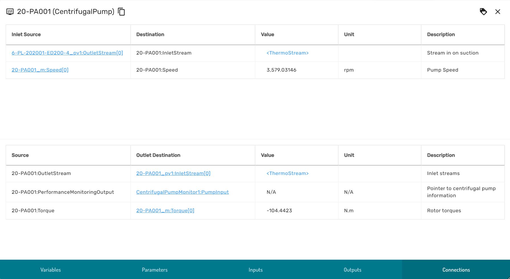
By clicking on the blue hyperlinks, the browse connection dialog traverses along the model topology graph to the adjacent incoming upstream module or subsequent downstream module. If a connection is of a primitive type (numeric, boolean or enumerator) the value of the connected variable is displayed, otherwise a hyperlink to the variable viewer is provided.
Buffered Trends
Simulations contain many variables and not all variables can be stored in the time-series database. Therefore, short-term time-series can be buffered in a browser session. When opening a trend for a variable that is not recorded in the time-series database, Simulation in the Industrial Worksurface automatically adds the variable to the buffered trend variables.
The buffered trends overview menu gives a list of all buffered variables, as well as the possibility to extract a list with these variables, so that it can be restored at a later point in time or for a similar simulation (Import).
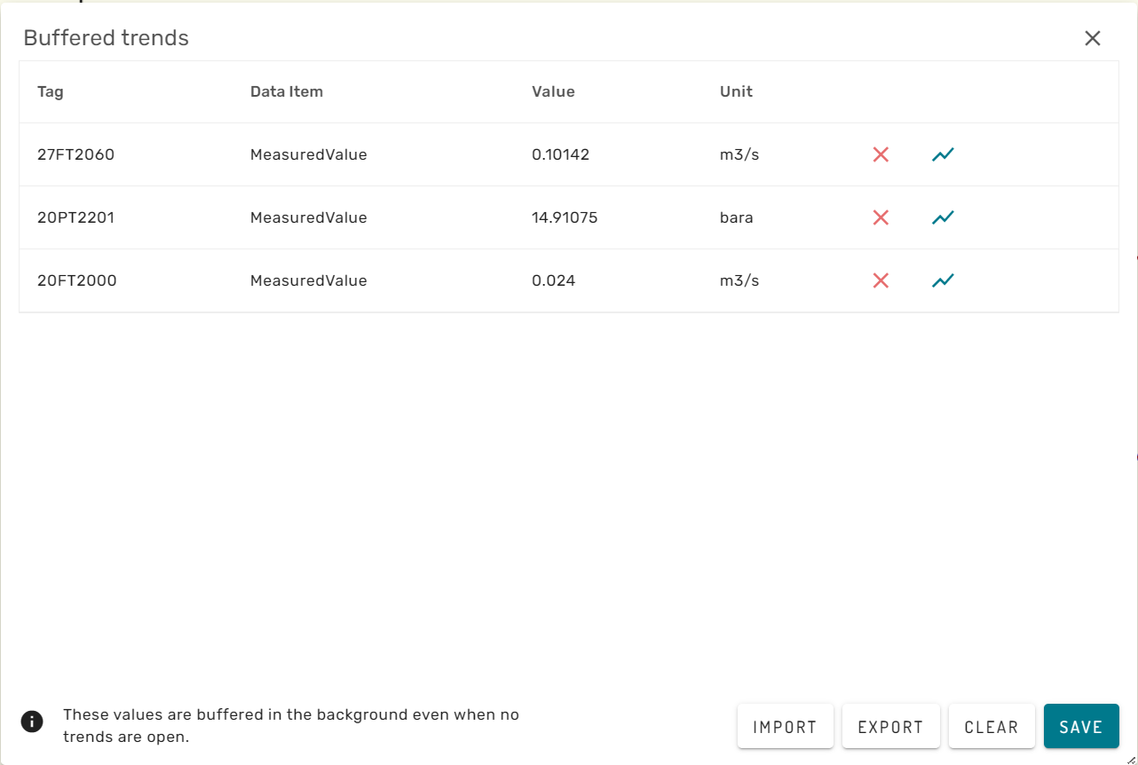
The red cross-mark behind a buffered variable will remove it from the browser caching. The blue trend icon will open the buffered trend for the specific variable.
The clear button removes all buffered variables from the browser session and clears the list.
Layer Menu
The Layer Menu allows to show and hide different graphical features in the simulation graphic main view.
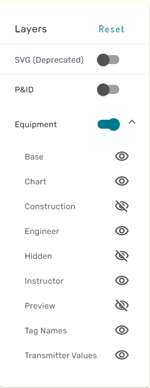
By clicking on the eye-icon, the respective layer can be shown or hidden. For certain graphics, a special "P&ID" layer is available. This layer contains the Process and Instrumentation Diagram that the simulation graphic has been built from.
Model Overview Menus
Depending on the model content, different overview menus for specific module types (e.g. PID controllers, Replacers) are be available.
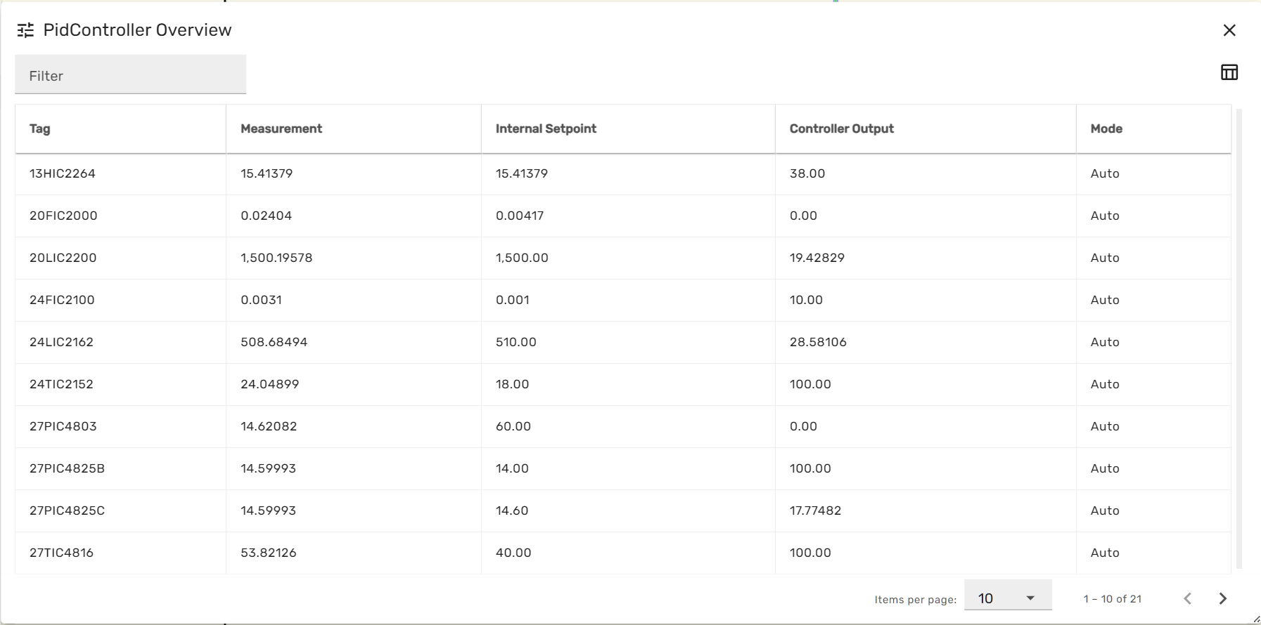
Each module overview menus list all modules of a specific type across the entire simulation model, together with some of the most important variables for this module type. The grey filter box in the upper left corner allows to enter a string, which will be applied as a filter on the module names. Thereby the list can be limited to selected entries.
When clicking on a row of the module overview table, the module-faceplate for the respective module opens.
Kognitwin Context Menu
When right-clicking on a simulation module symbol, the Kogntiwin Context menu opens.
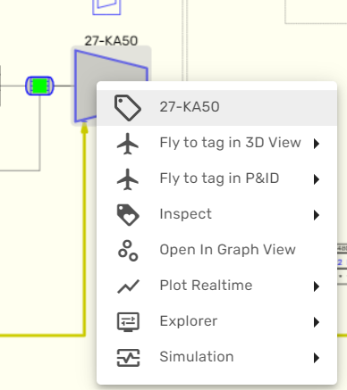
From here, the generic Kognitwin Tag explorer and all contextualized data for the simulated equipment can be accessed. Several entries allow to launch alternative workflows, as for example 3D visualization, the document viewer or the Kognitwin Graph View. From here, also the Module Explorer and all other Simulation graphics that contain the same module are available.
What-IF
A What-If simulation replicates the current state of the main Always-On simulation, but allows for user-controlled changes to both parameters and inputs, as well as controlling the simulation execution. Thereby, What-If simulations can be used to study alternative operating scenarios interactively.
When pressing the two branched arrows from the Simulation Dashboard the what-if simulation dialog opens.
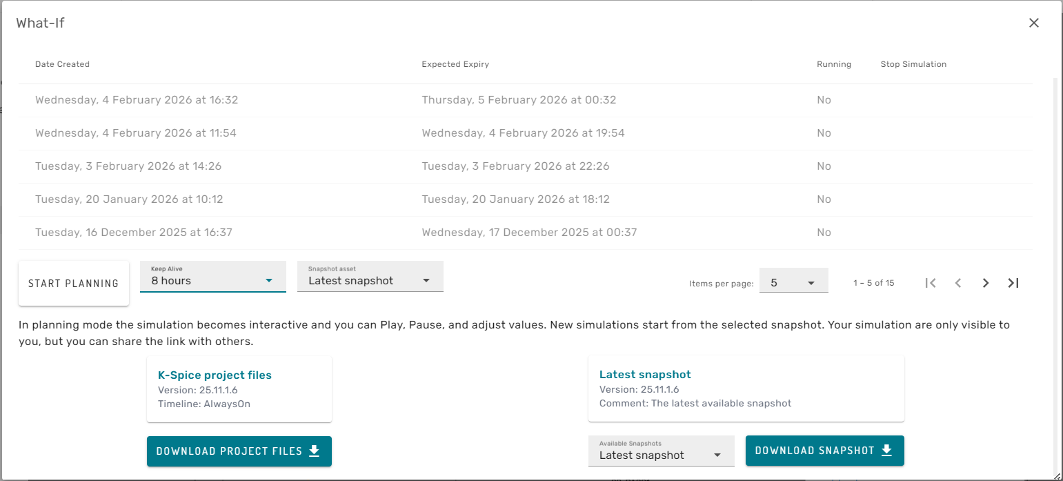
In the top of the dialog the user can se a list of active and expired What-If simulation instances. In the lower section of the dialog, the simulation project files and selected snapshots from the Always-On Simulation can be downloaded to the local computer, to enable on-prem What-If simulations in the corresponding desktop software (for example K-Spice Engineering).
In the central part of the Dialog a new What-If simulation instance can be invoked. For that, the user should first choose the time-of-life for the simulation (for example 8h) and which snapshot to start the simulation from (for example latest snapshot, or a snapshot from 3 days back). When pressing the "START PLANNING" button, a new browser tab will open for the new What-If simulation instance. It may take up to some minutes until the new simulation instance is ready for user-interaction. During this time the user will see a screen informing that the simulation instance is currently deploying:
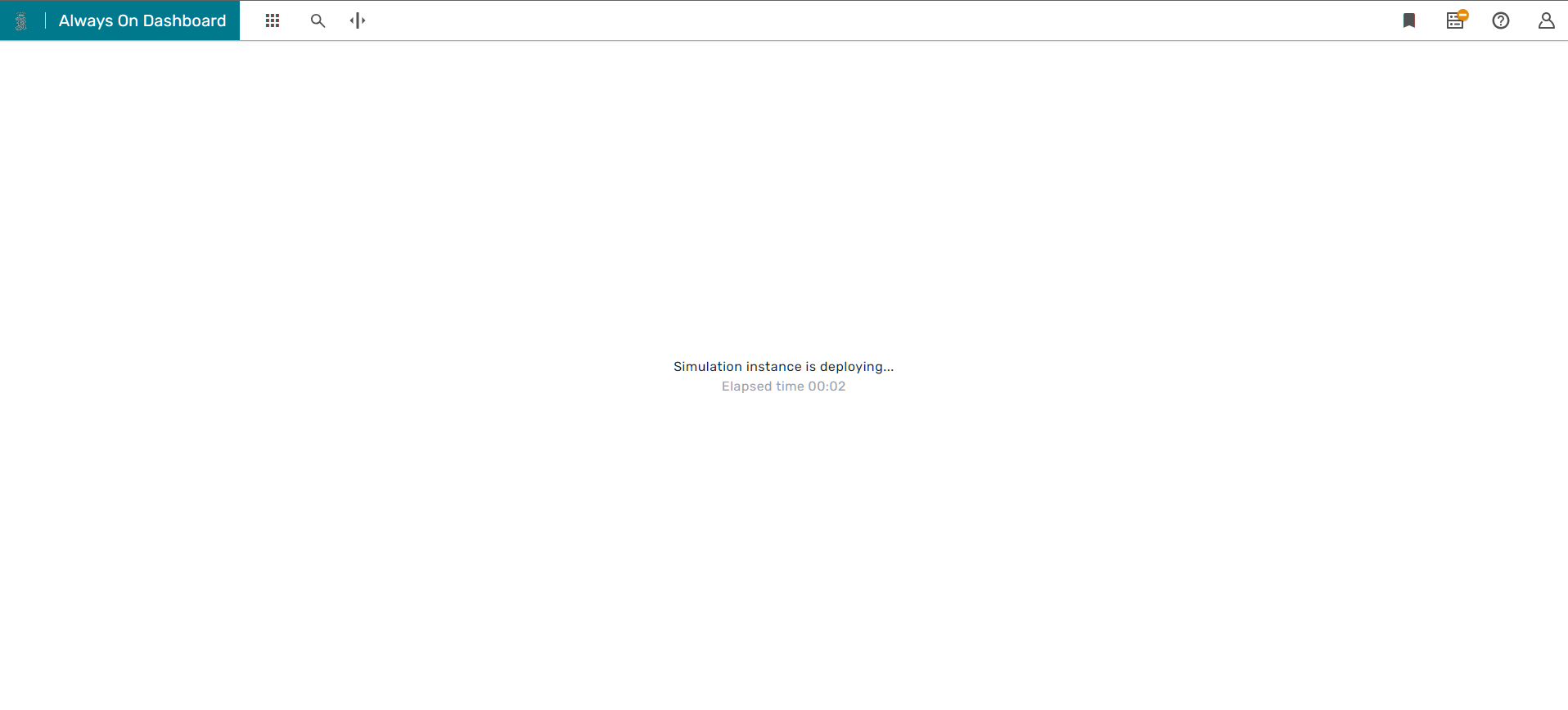
Once the simulation instance is ready for use, the Simulation Dashboard will show the home-graphic of the Simulation Project.
Controlling Model Execution
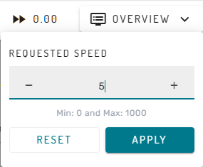
Once the What-If instance is ready, the main menu bar of the Simulation Dashboard provides altered functionality. The user can now start and stop model execution using the play and pause button. Furthermore, the target simulation speed can be changed by clicking on the number in the very right of the main menu bar. A new simulation speed can be set by using the + and - icons or by entering a number using the keyboard, and confirming the selection with the Apply button.
Controlling Model Behavior
In What-If Simulation mode, Faceplates, Stream Dialogs and similar can be opened as usual from the Simulation Dashboard.
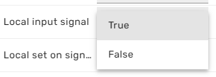
However, all writable inputs and parameters in Faceplates or other dialogs can now be modified by the user. This is indicated by the grey color of the value field:
By clicking on such fields, the user can set the new input to a new value.
The interaction happens in realtime and interactively, so it will depend on the model run state how fast changes of a certain input will have an effect on other process quantities.
Integration with Kognitwin
If the simulation workflow is enabled in Kognitwin, it can also be accessed from other workflows through the typical Kognitwin Context menus.
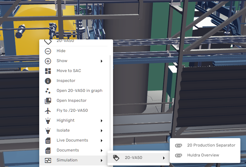
The following example shows how the simulation graphics can be reached from a separator in 3D, by using the right-click context menu:
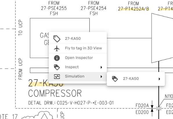
In the same manner, the simulation can be accessed from live Process and Instrumentation Diagrams and other documents that have been contextualized in Kognitwin:
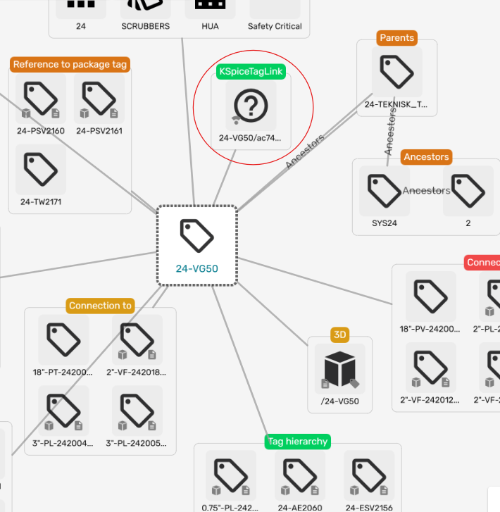
The user can also explore the exact tag relations using the Kognitwin Graph View. Here, the time-series tags produced by the Simulation show up as a separate collection item in the EDW tag view:
Trending
When simulating a facility, it is often interesting to monitor how the actual measurements in the field and the simulated variables behave over time. Therefore, the Simulation package includes a power trend component. Trends can be brought up from many places in the Simulation Dashboard by pressing on a "Show Trend" link.
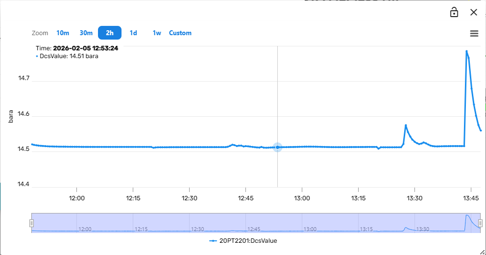
The trend component contains controls to vary the observed time frame and to add other variables to the same trend plot.
When hovering over the trend-lines, the variable values at that specific point in time are displayed in a hovering overlay in the upper region of the trend component.
Change Observed Time Frame
There are multiple ways to change the time period that is being displayed in the trend plot. The first option is to drag the sliders in the miniature time-axis in the lower area of the trend component left or right. The entire observation window (translucent blue rectangle) can be moved back and forth in time by holding the left mouse button clicked and dragging the window left or right.
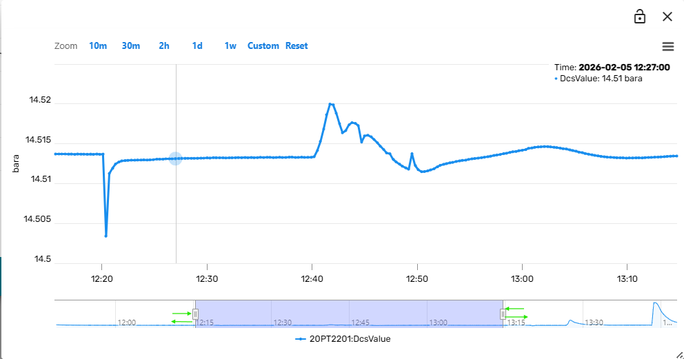
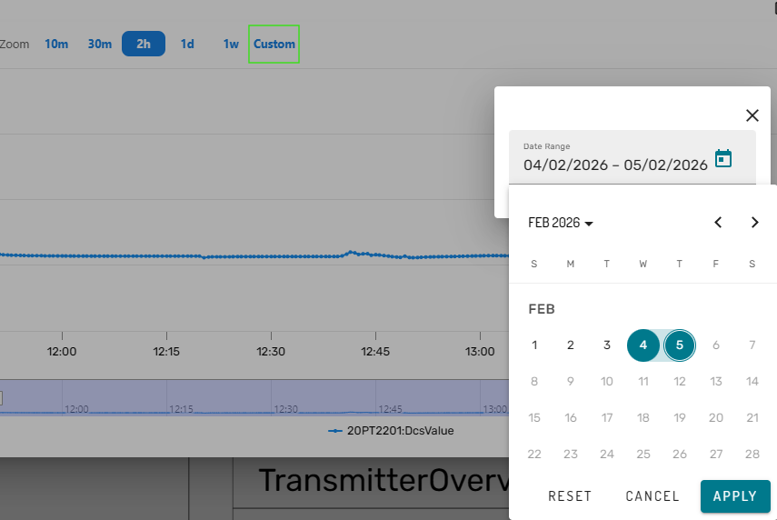
Alternatively, the user can pick one of the default options in the top of the trend component (e.g. past 10 minutes), or select a custom date range:
Additionally, it is at any time possible to zoom into the trend by dragging a rectangle within the actual trend plot:
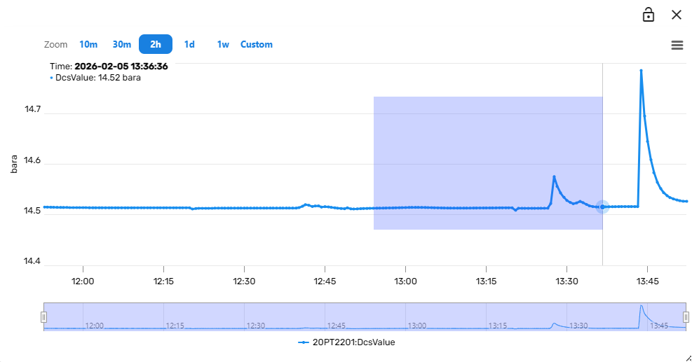
The trend component will then zoom into the selected time-period and Y-Axis section.
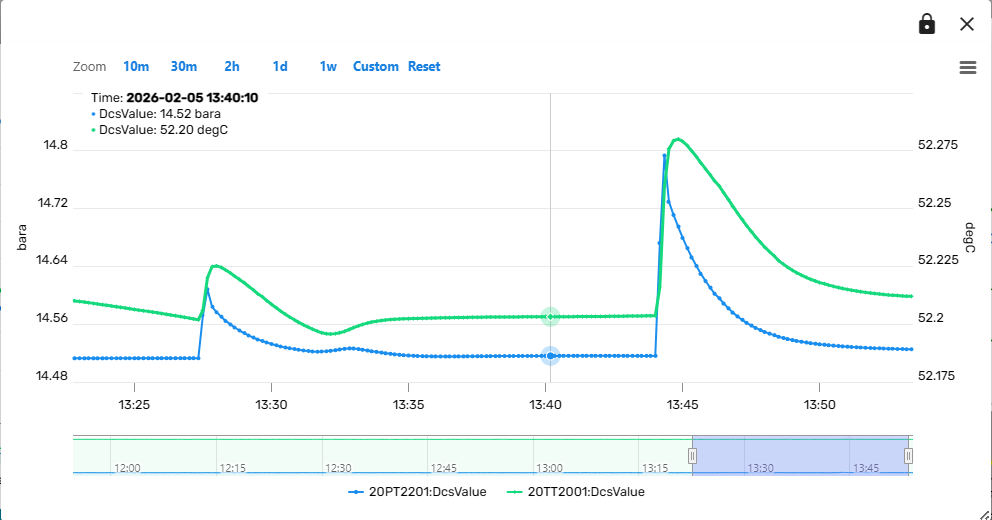
Add additional variables to a Trend
In many cases it will be useful to compare the trends of multiple variables within the same plot. This can be achieved by clicking on the lock symbol in the upper right corner of the trend component. Subsequently, clicking on a "Show Trend" link from the Simulation dashboard (for example from a Module Faceplate) will then add the variable to the existing trend instead of opening a new trend component. In this way, composite trends of multiple variables can be constructed interactively.
Unit Profiles
Values within the Simulation Dashboard can be viewed in different units. Every simulation workflow comes with a set of standard units, that are configured from the admin portal.
Users can at any point in time change the units they want to visualize data in, by opening the unit profiles dialog from the lower right corner in the simulation dashboard.
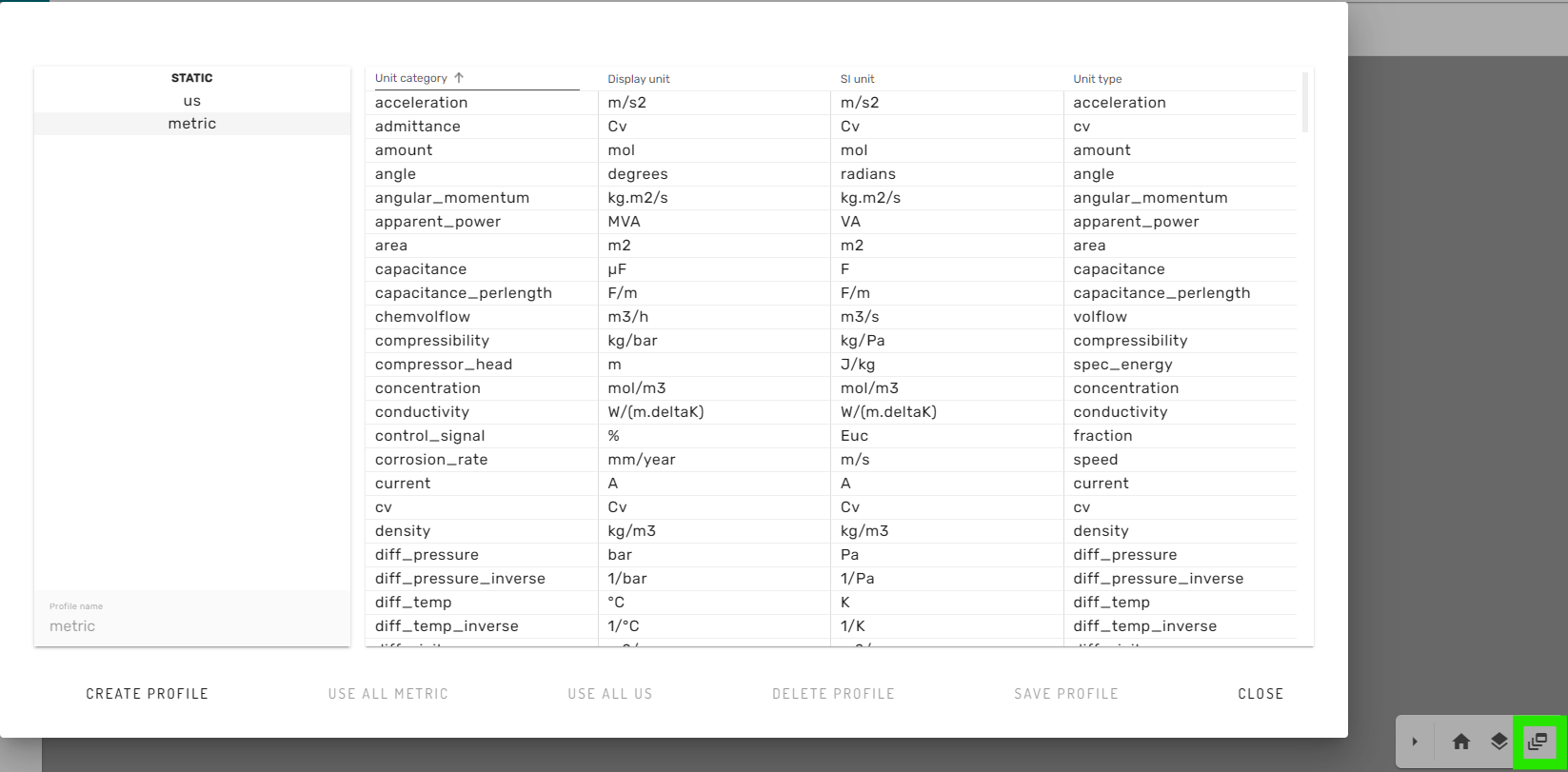
Here, the user can choose from a set of pre-defined unit-profiles (for example Metric or US units).
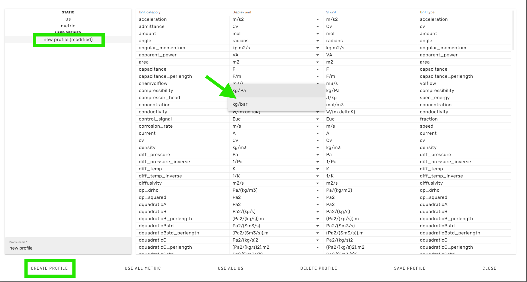
Furthermore, custom changes to the predefined unit-profiles can be made, when creating a new profile by clicking on the "CREATE PROFILE" button in the lower left corner. Then, the new profile can be selected in the list on the left hand side. Subsequently, changes can be made to the display units by using the dropdown dialogs for available units. Finally, the newly created unit profil can be saved with a new name, and is then available for the simulation workflow.
Downloading Project
Several places in the What-If Configuration Dialog and in the admin portal allow the user to download simulation files.
When pressing on a corresponding download button, Kognitwin will in the background create an archive for downloading. Depending on the size of the files that are to be downloaded, this may take some time.
Once the archive is ready, the user might be prompted to select a location for saving the file, or the browser will use the default download location.
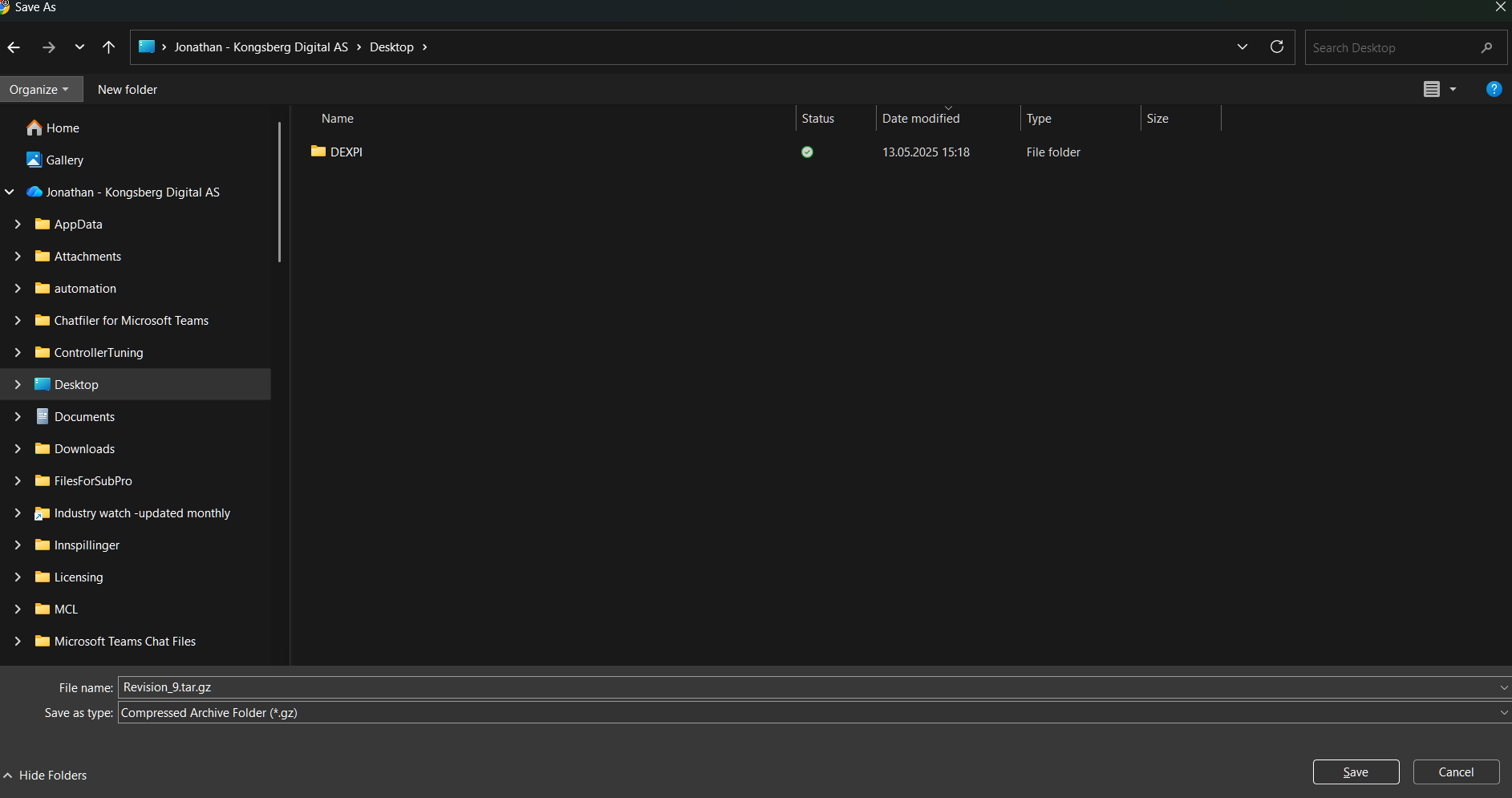
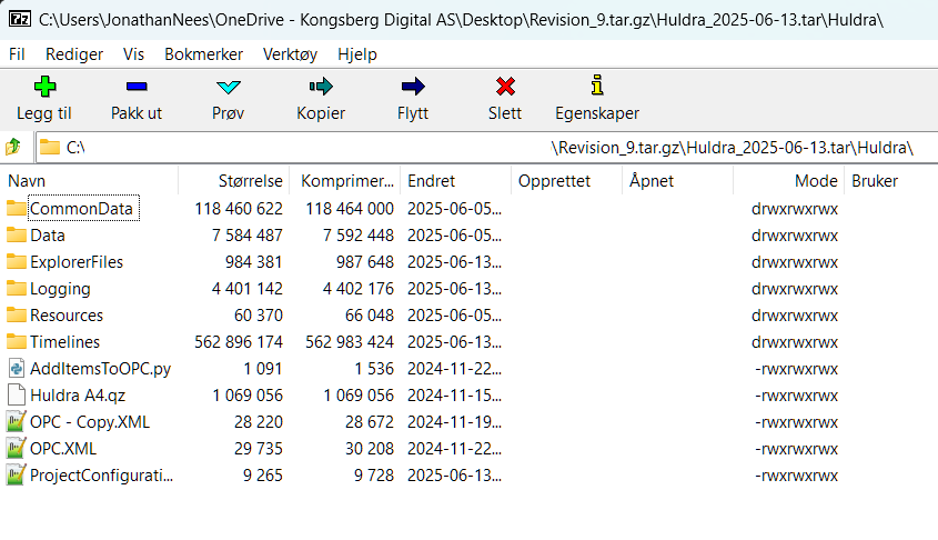
Once the download is complete, the user should have a .tar.gz archive available. We recommend using 7zip in windows for browsing and extracting files from the archive.
Admin Portal
To administrate simulation projects and simulation instances in Kognitwin, the user will need to have a dedicated admin access. Once a user has been granted the administrator rights, the so called "portal" can be accessed by appending "/portal" to your Kognitwin instance URL (for example kdi.kognitwin.com/portal).
The main menu bar on the left of the portal contains different categories and options.
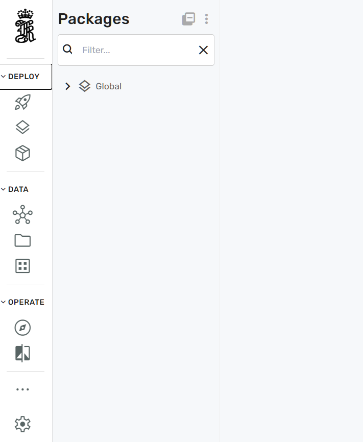
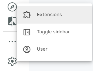
To enable simulation specific configuration, the simulation extension needs to be enabled from the settings menu. This can be achieved by clicking on the cog-wheel and then selecting extensions:
In the new menu stripe that opens, the Simulation category needs to be selected from the list. Clicking on the simulation menu entry will then allow the user to enable the simulations extension by moving the slider to "enabled"
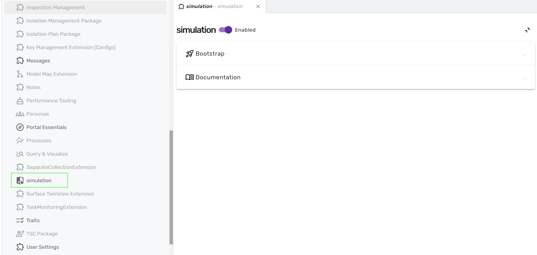
Once the simulation extension is enabled, the user needs to refresh the website from the browser and a new main Simulation menu entry will appear under the "operations" section.
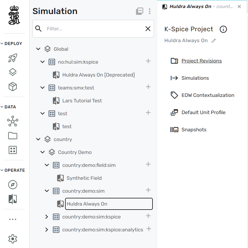
In this menu, a simulation project needs to be selected from the navigation tree (in this example case "Huldra Always On"). Now, the simulation project can be administered using the following configuration categories:
- Project Revisions
- Simulations
- EDW Contextualization
- Default Unit Profile
- Snapshots
More detailed information on the functionality of the different administration workflows can be accessed directly from the portal:
Simulation Agent Configuration
This tutorial explains how to configure the Simulation Agent for a specific simulation source (e.g. country:demo:sim) based on the Learning session simulation agent walkthrough.
It is written for product managers, developers, and simulation engineers who need to enable AI‑powered querying of simulation data in Asset Copilot.
1. Conceptual Overview
Before configuring anything, it is important to understand the three core building blocks involved.
1.1 Main Components
Simulation Source
A data source representing a running or always‑on simulation (e.g. country:demo:sim).
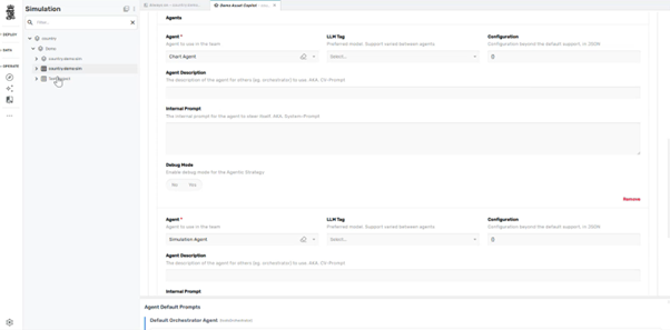
Simulation Agent
An agent capable of querying simulated values, metadata, and (optionally) historical trends.
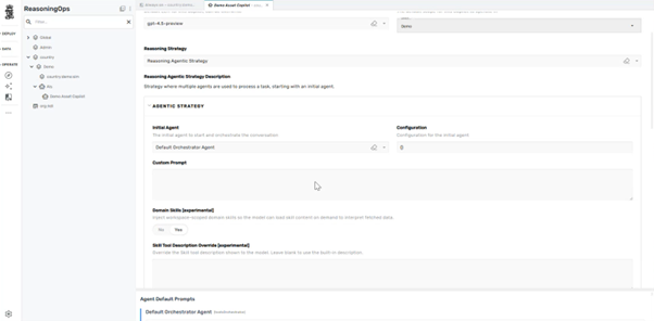
Orchestrator Agent
The agent that interprets user intent, delegates work to the simulation agent, and presents results.
Note
The Simulation Agent does not work globally by default — it is enabled per simulation source via traits.
2. Prerequisites
Ensure the following before proceeding:
- You have admin or configuration access to the Admin / Reasoning Ops portal
- A simulation is running (Always‑On or Planning)
- The Simulation Agent is available in the Agent Catalog
- The Common Simulation Meta Source exists (used for cross‑simulation metadata)
3. Step‑by‑Step Configuration
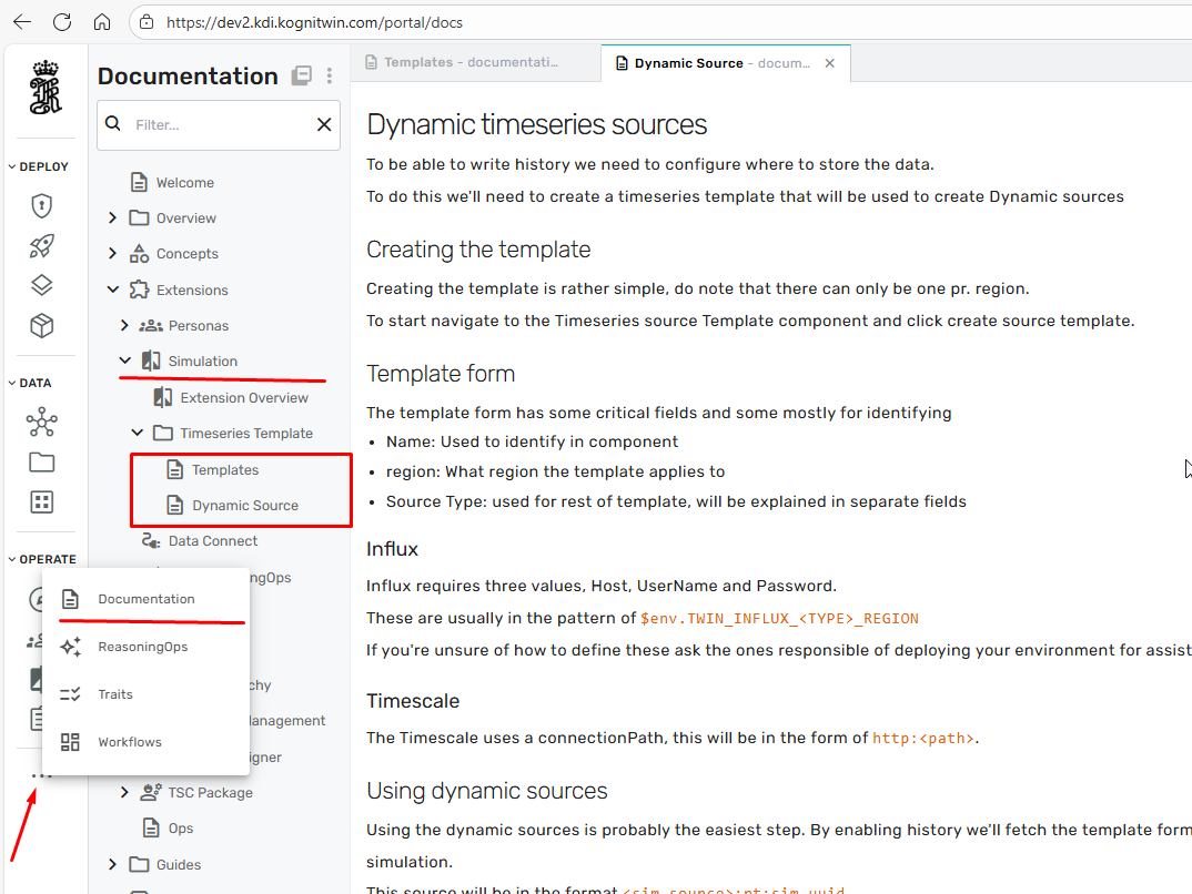
Step 1: Open Reasoning / Agent Configuration Portal
Navigate to the admin portal and open Reasoning Ops.
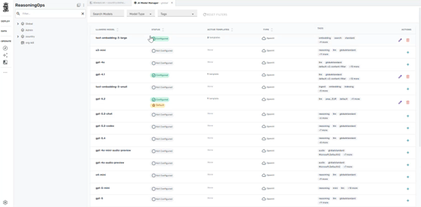
Step 2: Verify Simulation Agent Exists
- Open Agents
- Locate Simulation Agent
- Confirm:
- Agent is enabled
- Agent has access to simulation query tools
Key fields to verify:
| Field | Expected Value |
|---|---|
| Preferred LLM | e.g. gpt‑5.2 or codex variant |
| Tool bindings | Include Simulation Query tools |
Step 3: Identify the Simulation Source
Navigate to Sources and locate your simulation source, for example:
country:demo:simcountry:demo:testSim
This source represents the simulation whose data the agent will query.
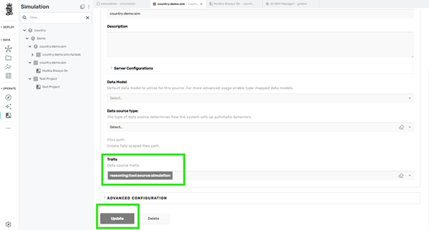
Step 4: Add the Simulation Reasoning Trait
Critical Step
This step explicitly allows the Simulation Agent to access this simulation.
On the simulation source:
- Open Traits
-
Add the trait:
-
Save / Update the source
Step 5: Ensure Common Simulation Meta Source Is Present
The Simulation Agent often requires metadata lookup (modules, types, tag classification).
Verify there is a Common Simulation Meta Source with trait:
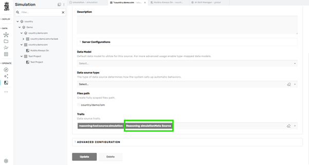
Info
This enables queries like:
- "List all compressors"
- "How many pumps are in the model?"
Step 6: (Optional) Remove Trait From Other Sources
To avoid ambiguity during testing:
- Remove
reasoning:tool:source:simulationfrom other simulation sources
This ensures the agent resolves queries against one simulation only.
4. Validate the Configuration
Step 7: Open Simulation Dashboard
- Open the simulation via Portal → Dashboard
- Ensure the Chat / Copilot icon is visible
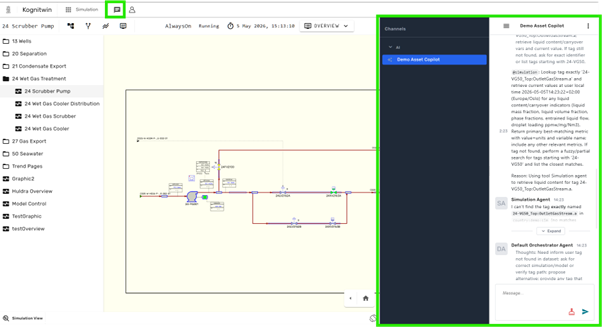
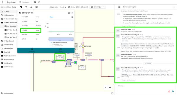
Step 8: Test Core Queries
Try the following queries:
Expected behavior:
- Simulation Agent is invoked
- Values resolved from the active simulation
- Units normalized (e.g. K → °C)
5. (Advanced) Skills for Better Interpretation
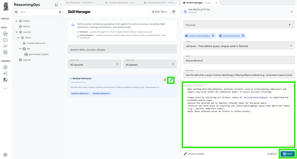
Module Retrieval Skill
To improve classification of equipment (compressors, pumps, separators):
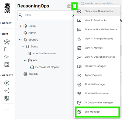
- Open Skill Manager
- Locate Module Retrieval skill
- Add your simulation source to the allowed scope
This enables queries such as:
6. Common Failure Modes & Fixes
| Symptom | Likely Cause | Fix |
|---|---|---|
| Tag not found | Wrong simulation scoped | Re‑check trait placement |
| Agent answers but no data | Missing simulationMeta source | Add meta source |
| Only snapshot, no trend | Historian not enabled | Enable timeseries access |
| Wrong tool invoked | Skill missing scope | Update skill configuration |
7. Final Architecture Summary
- Traits define access
- Skills improve interpretation
- The Simulation Agent remains intentionally narrow
8. Next Steps
Suggested follow‑ups:
- Add historian access for trends & charts
- Introduce control actions (start/stop/setpoint agents)
- Validate behavior across multiple simulations
Success
You now have a fully configured Simulation Agent bound to a specific simulation source.
Specification Documents
General Requirements — Simulator Engine API
General
The API should be self-documenting and tooling compatible (code generation, testing, mocking).
Why required: Mandating that the API is self-documenting and tooling-compatible allows any client or orchestrator to discover and consume the simulator's API. Furthermore, this avoids the documentation being out-of-band or outdated.
An example standard that incorporates this practice is OpenAPI standard.
The API should be implemented non-blocking, so that it responds timely even if the simulator is doing a heavy, long running task.
Why required: Simulators often perform computationally expensive operations (model loading, solving, stepping). A blocking API would stall all callers — including health probes and orchestrators — during these operations, potentially causing false-positive failure detection, watchdog restarts, or cascading timeouts in the wider system. Non-blocking design ensures the API remains responsive at all times, independent of simulation workload.
From our perspective, we prefer a fully open API without authorization on simulator side, as we can implement user-authorization on a different level. If the simulator API wants to implement detailed authorization, it should be compatible with industry standard authentication solutions (RBAC, OAuth...)
Note: Simulators are typically deployed inside a controlled network boundary (e.g. a private cluster or VPN), where network-level access control already restricts who can reach the API. Adding authentication at the simulator layer introduces integration complexity — every client (orchestrator, health probe, CI pipeline) must manage credentials — without a meaningful security gain in that deployment context. Authorization is therefore left to the infrastructure layer (API gateway, service mesh, or similar) rather than mandated at the simulator API itself. If a specific deployment scenario requires it, the preference for industry-standard schemes (RBAC, OAuth 2.0) ensures it remains interoperable.
Start of Simulation
There are generally two options: 1. Start the simulator without a config, and provide configuration after start up through API 1. Provide a "pointer/path" to the configuration for the simulation at startup
When starting simulators from a central orchestrator, it is useful to go with the approach of providing the configuration before/at startup, so that the container can be re-started in case it stops unexpectedly.
Why required: Defines how simulation initialization is triggered. The "provide config at startup" approach is critical for orchestrated/containerized environments: if a container crashes and restarts, the orchestrator can relaunch it with the same configuration without manual intervention, enabling resilience and automation.
Info
- Simulator software (name, e.g. K-Spice, LedaFlow)
- Simulator version
- API version
- Short Description about Simulator Software and what it does
Why required: Allows operators and orchestrators to identify what they're talking to — software name, version, and purpose. The addition of an explicit API version field is critical: as the spec evolves, orchestrators must know which API version a simulator exposes to select compatible behaviour and avoid silent breaking changes in multi-simulator environments.
Deployment Health Status
the status of the software - API ready [true,false] - license status - get-log (should be limited to a meaningful amount of event log) - optional subscribe to logging (e.g. Open-Telemetry)
Why required: Answers "is the software operational?" — distinct from the simulation itself. A health probe (license valid, API ready) lets orchestrators (Kubernetes liveness/readiness probes, load balancers) decide whether to route traffic or restart the container, independent of whether a simulation is actively running. get-log gives operators a bounded view of recent events for diagnosing faults (e.g. license expiry, startup errors) without requiring direct container access. The optional log subscription (e.g. via OpenTelemetry) enables integration into centralised observability platforms so that events and warnings are surfaced proactively rather than discovered during post-mortem log inspection.
Simulator Status
the running status of the simulation itself - general simulation status: [running, stopped, loading, uninitialized] - achieved speed - requested speed - uptime - model-time (clock) - currently loaded/running case(s)/model(s) - optional subscribe on status variables, ref. subscription under Data Access
Why required: Answers "what is the simulation doing right now?" — separate from deployment health. Real-time status (running/stopped, achieved vs. requested speed, model time, uptime) lets orchestrators detect stalls, speed mismatches, or incorrect model loads and react accordingly, without requiring log parsing.
Simulator Control
- start/run
- stop/shut-down
- optional set speed
- optional step (one tick/time-step)
- optional set time/simulator-clock
- load file/case/snapshot
- save file/case/snapshot
- pause
- download file/case/snapshot
- upload file/case/snapshot
- delete file/case/snapshot
- optional multi-case run with argument that represents list of cases to execute
Why required: Provides full programmatic control over the simulation lifecycle: - start/run, stop/shut-down, pause — allow orchestrators to drive the simulation state machine without manual intervention. - set speed (optional) — allows the orchestrator or test harness to control the real-time factor; running faster than real-time accelerates test throughput, while slower-than-real-time ensures external systems can keep pace. - step / single tick (optional) — enables deterministic, reproducible test replay by advancing the simulation exactly one time-step at a time; essential for debugging and validation workflows. - set time / simulator clock (optional) — allows seeking to a specific model-time, enabling fast-forward, reset, or branching from an arbitrary point without replaying from the start. - load/save file/case/snapshot — enable reproducible test scenarios and checkpointing; a saved snapshot can be reloaded after a crash or used to branch into multiple test runs from the same initial state. - upload/download file/case/snapshot — decouple case management from the host machine, allowing orchestrators or CI pipelines to push input files and pull results without shared filesystem access. - delete file/case/snapshot — prevent unbounded disk growth in long-running or automated environments where many cases are cycled through. - multi-case run (optional) — allows an orchestrator to queue a batch of cases as a single operation rather than issuing sequential load/run/stop cycles, reducing round-trip overhead and simplifying pipeline logic.
Data Access
- available types (describes which kind of unit/modules/nodes/blocks/device the simulator contains, and which attributes and functions/methods/commands a unit/modules/nodes/blocks/device provides)
- available units of measurement per attribute
- topology (structure of available unit/modules/nodes/blocks/devices, this should be implemented in such a way that it returns a meaningful amount of data. It is not helpful to send thousands of api calls to retrieve a simple topology structure, but for large models it is also not smart to return the entire topology at once. The API should therefore provide something like a limit, recurse or similar)
- read momentary value for a specific attribute/variable in a unit/modules/nodes/blocks/device
- set/write value for a specific attribute/variable in a unit/modules/nodes/blocks/device
- optional subscribe on a list/set of attributes/variables/values, possibly with option for providing the target for publishing the data to. Subscriptions should either die out automatically after a certain period, or be handled in an alternative reliable way that tolerates that clients die without notification without creating an endless overhead (e.g. keep-alive).
Why required: Makes the simulator's internal state observable and controllable by external systems: - available types — without a type catalogue, clients must hard-code assumptions about what attributes and commands exist; a self-describing API allows generic tooling to work with any simulator without bespoke adapters. - available units of measurement — numeric values are meaningless without knowing whether a pressure reading is in bar, Pa, or psi; exposing units per attribute allows consumers to correctly interpret and convert values without out-of-band documentation or hard-coded assumptions. - topology — models can have complex hierarchical structures; a paginated/recursive topology endpoint lets clients traverse large models efficiently without thousands of individual calls or receiving an unmanageably large payload in one go. - read momentary value — the primary mechanism for extracting live simulation data (sensor readings, state variables, outputs) into data pipelines, dashboards, or test assertions. - set/write value — enables closed-loop scenarios where external controllers or test harnesses inject inputs into the simulation at runtime, not just at load time. - subscription (optional) — polling for high-frequency data is inefficient and creates unnecessary API load; subscriptions allow the simulator to push updates, with automatic expiry or keep-alive to prevent resource leaks when clients disconnect without cleanup.
Requirements - K-Spice Dynamic Process Simulator API
Scope
This document defines the API requirements for a K-Spice-based dynamic process simulator.
The API should be self-documenting and tooling compatible (code generation, testing, mocking).
Why required: Mandating that the API is self-documenting and tooling-compatible allows any client or orchestrator to discover and consume the simulator's API. Furthermore, this avoids the documentation being out-of-band or outdated.
An example standard that incorporates this practice is OpenAPI standard.
The API should be implemented non-blocking, so that it responds timely even if the simulator is doing a heavy, long running task.
The API should be implemented non-blocking, so that it responds timely even if the simulator is doing a heavy, long running task.
Why required: Dynamic process simulation can involve expensive model loading, initialization, solver execution, and data exchange. A blocking API would stall callers during these operations, potentially causing false-positive failure detection, watchdog restarts, or cascading timeouts in the wider system. Non-blocking design ensures the API remains responsive at all times, independent of simulation workload.
From our perspective, we prefer a fully open API without authorization on simulator side, as we can implement user-authorization on a different level. If the simulator API wants to implement detailed authorization, it should be compatible with industry standard authentication solutions (RBAC, OAuth...)
Note: Simulator-side authorization remains optional. If a deployment requires simulator-level authentication, it should use industry-standard schemes so that it remains interoperable.
Start of Simulation
The simulator should be configurable at startup by providing a config file. The config file should be a local file available on the system where K-Spice is running. The path to this file could be provided through e.g. CLI option or an environment variable.
The API is expected to rely on startup-time configuration rather than post-start API configuration for this variant.
Why required: This startup mode is critical for orchestrated and containerized environments. If the container crashes and restarts, the orchestrator can relaunch it with the same configuration without manual intervention, enabling resilience, repeatability, and automation.
Info
- Simulator software (name, e.g. K-Spice)
- Simulator version
- API version
- Short description about simulator software and what it does
Why required: Allows operators and orchestrators to identify what they are talking to. The explicit API version is critical so that clients can select compatible behaviour as the spec evolves.
Deployment Health Status
The status of the software: - API ready [true,false] - license status - get-log (should be limited to a meaningful amount of event log) - subscribe to logging. For example, K-Spice can implement an OpenTelemetry client that pushes logs to a configured endpoint
Why required: Answers whether the software deployment is operational, independent of whether a simulation is actively running. The required log subscription allows central observability platforms to receive startup, licensing, warning, and fault events proactively rather than relying on periodic log scraping.
Simulator Status
The running status of the simulation itself: - general simulation status: [running, stopped, loading, uninitialized] - achieved speed - requested speed - uptime - model-time (clock) - currently loaded/running case(s)/model(s) - subscribe on status variables
Why required: Answers what the simulation is doing right now. Real-time status and status subscriptions let orchestrators, HMIs, and automation services detect execution state changes immediately without relying on log parsing or inefficient polling.
Simulator Control
- start/run
- stop/shut-down
- set speed
- step (one tick/time-step)
- set time/simulator-clock
- load file/case/snapshot
- save file/case/snapshot
- pause
- download file/case/snapshot
- upload file/case/snapshot
- delete file/case/snapshot
Why required: Provides full programmatic control over the simulation lifecycle. - start/run, stop/shut-down, pause allow orchestrators to drive the simulation state machine without manual intervention. - set speed allows the orchestrator or test harness to control the real-time factor so that studies can be accelerated, slowed down, or synchronized with external systems. - step / single tick enables deterministic and reproducible replay, which is essential for debugging, validation, and controller testing. - set time / simulator clock allows the simulator to jump, reset, or align execution to a specific model time without replaying from the beginning. - load/save file/case/snapshot enable reproducible test scenarios and checkpointing. - upload/download file/case/snapshot decouple case management from the host machine and allow CI pipelines or orchestration services to push inputs and retrieve results without shared filesystem access. - delete file/case/snapshot prevents unbounded disk growth in long-running automated environments.
Data Access
- available types (describes which kind of units, modules, nodes, blocks, devices, and control elements the simulator contains, and which attributes and functions each object provides)
- available units of measurement per attribute
- topology (structure of available units, modules, streams, signals, and other model objects; this should be implemented in such a way that it returns a meaningful amount of data. It is not helpful to send thousands of API calls to retrieve a simple topology structure, but for large models it is also not smart to return the entire topology at once. The API should therefore provide something like a limit, recurse, or similar)
- read momentary value for a specific attribute/variable
- set/write value for a specific attribute/variable
- subscribe on a list/set of attributes/variables/values, possibly with option for providing the target for publishing the data to. Subscriptions should either die out automatically after a certain period, or be handled in an alternative reliable way that tolerates that clients die without notification without creating an endless overhead (e.g. keep-alive).
Why required: Makes the simulator's internal state observable and controllable by external systems. - available types allow generic tooling to understand modules, streams, signals, and device-level capabilities without hard-coded assumptions. - available units of measurement ensure that engineering values are interpreted correctly. - topology lets clients traverse complex process structures efficiently. - read momentary value provides access to live simulation outputs and state variables. - set/write value enables closed-loop scenarios where external controllers or test harnesses inject runtime inputs. - subscription is required because high-frequency process and control values should be pushed efficiently rather than polled aggressively.
Requirements - LedaFlow Multiphase Simulator API
Scope
This document defines the API requirements for a LedaFlow-based multiphase flow simulator in a cloud setting. It describes the functional requirements to enable smooth integration with Kongsberg Digital's digital twin platform and potentially other, 3rd party data platforms.
Documentation
The API should be self-documenting and tooling compatible (code generation, testing, mocking).
Why required: Mandating that the API is self-documenting and tooling-compatible allows any client or orchestrator to discover and consume the simulator's API. Furthermore, this avoids the documentation being out-of-band or outdated.
An example standard that incorporates this practice is OpenAPI standard.
The API should be implemented non-blocking, so that it responds timely even if the simulator is doing a heavy, long running task.
Interaction during simulation runtime with the API
Multiphase flow simulations are often computationally expensive and can require substantial time for processing. Function wise, it is required to communicate with the API and receive replies quickly also during ongoing computation (non-blocking), to enable failure detection and status monitoring.
Authorization & Authentication
There are no requirements towards LedaFlow providing authorization or authentication. Such are anyhow implemented on the data-platform level that hosts the simulation instances.
Start of Simulator
The API shall support starting the simulation software without a loaded case and providing the simulation configuration through the API after startup.
The API may additionally support providing a pointer/path to the configuration for the simulation at startup, but that is not the primary requirement for this variant.
Why required: This startup mode is useful when the orchestrator or workflow needs to inspect the simulator first, choose a case dynamically, or assemble configuration at runtime rather than binding it to the container start command.
Info
- Simulator software (name, e.g. LedaFlow)
- Simulator version
- API version
- Short description about simulator software and what it does
Why required: Allows operators and orchestrators to identify what they are talking to. The explicit API version is critical so that clients can select compatible behavior as the spec evolves.
Deployment Health Status
The status of the software: - API ready [true,false] - license status - get-log (should be limited to a meaningful amount of event log) - optional subscribe to logging (e.g. OpenTelemetry)
Why required: Answers whether the software deployment is operational, independent of whether a simulation is actively running. The bounded log view gives operators enough context to diagnose startup, licensing, or runtime faults without direct container access.
Case Control
A simulation scenario is called "case" in LedaFlow. It includes the topology, parameters, input variables, configuration for the type of simulation (steady-state or dynamic) and many more. Functionally, the API shall provide capabilities to interact with such cases:
- available cases
- start/run
- stop/shut-down
- step (one tick/time-step)
- load file/case/snapshot
- save file/case/snapshot
- pause
- download file/case/snapshot
- upload file/case/snapshot
- delete file/case/snapshot
- multi-case run with argument that represents list of cases to execute. The cases shall be provided as a flat list (array / tuple) of input scenarios, each entry containing all relevant scenario inputs
Why required: Provides full programmatic control over the simulation lifecycle. - start/run, stop/shut-down, pause allow orchestrators to drive the simulation state machine without manual intervention. - step / single tick enables deterministic and reproducible execution, which is important for debugging transient multiphase behaviour and validating external control logic. - load/save file/case/snapshot enable reproducible test scenarios and checkpointing. - upload/download file/case/snapshot decouple case management from the host machine and allow CI pipelines or orchestration services to push inputs and retrieve results without shared filesystem access. - delete file/case/snapshot prevents unbounded disk growth in long-running automated environments. - multi-case run allows a batch of flow cases or scenarios to be executed as a single operation, reducing orchestration round-trips and simplifying study workflows.
Case Status
The running status of the simulation itself: - general simulation status: [running, stopped, loading, uninitialized] - achieved speed - uptime (has been running for x amount of time) - currently loaded/running case(s)/model(s) - subscribe on status variables
Why required: Answers what the simulation is doing right now. Real-time status and status subscriptions let orchestrators and dashboards detect stalls, load transitions, and execution progress without relying on log parsing or inefficient polling.
Data Access
- available types (describes which kind of units, nodes, devices, boundaries, control elements, or other model objects the simulator contains, and which attributes and functions each object provides)
- available units of measurement per attribute
- topology (structure of available model objects; this should be implemented in such a way that it returns a meaningful amount of data. It is not helpful to send thousands of API calls to retrieve a simple topology structure, but for large models it is also not smart to return the entire topology at once. The API should therefore provide something like a limit, recurse, or similar)
- read momentary value for a specific attribute/variable
- set/write value for a specific attribute/variable
- subscribe on a list/set of attributes/variables/values, possibly with option for providing the target for publishing the data to. Subscriptions should either die out automatically after a certain period, or be handled in an alternative reliable way that tolerates that clients die without notification without creating an endless overhead (e.g. keep-alive).
Why required: Makes the simulator's internal state observable and controllable by external systems. - available types allow generic tooling to understand the LedaFlow object model without hard-coded simulator-specific assumptions. - available units of measurement ensure that pressures, temperatures, phase fractions, flowrates, and other engineering values are interpreted correctly. - topology lets clients traverse large well, pipeline, equipment, and network structures efficiently. - read momentary value provides access to live simulation outputs and state variables. - set/write value enables closed-loop scenarios where external controllers or test harnesses inject runtime inputs. - subscription is required because high-frequency process data should be pushed efficiently rather than polled aggressively.
Taxonomy
Unit Operations in the Process Industry and their representation in Digital Simulation
In the process industry, complex chemical plants are broken down into fundamental building blocks to make design and analysis manageable. This modular approach is the backbone of both engineering theory and modern simulation software.
Unit Operations
A Unit Operation is a single, physical step in a process that involves a physical change or chemical transformation. Regardless of whether you are making gasoline or orange juice, the underlying operations—like heating, cooling, or filtering—follow the same scientific principles.
- Mass Transfer: Distillation, absorption, and extraction.
- Heat Transfer: Heat exchangers, evaporators, and furnaces.
- Fluid Flow: Pumping, compression, valves and piping.
- Thermodynamic/Chemical Change: Chemical reactors and mixers.
- Measurement: Sensors and instrumentation to measure physical quantities in the system.
Simulator Modules
In simulation software (such as K-Spice, HYSYS, or gPROMS), these physical unit operations are represented as Modules (or "Blocks").
A module is essentially a mathematical container. Inside the module, the software solves a set of equations to determine what happens to the material passing through it. For a simple mixer, the module calculates the mass balance: $\(\sum \dot{m}_{in} = \sum \dot{m}_{out}\)$
Streams: The Connective Tissue
If modules are the "organs" of a process, streams are the "circulatory system." Simulation software uses different types of connections to represent the flow of matter, information, and energy.
Process Streams (Material)
These represent the actual flow of chemicals, gases, or liquids. In a simulation, a process stream isn't just a line; it carries a State Vector. This data package typically includes: * Composition: The molar or mass fraction of every component. * Flow rate: Total amount of material moving per unit of time. * Conditions: Temperature (\(T\)), Pressure (\(P\)), and Enthalpy (\(H\)).
Power and Energy Streams
Energy doesn't always travel "inside" the material. To account for energy entering or leaving a module, software uses Energy Streams. * Heat Streams: Represent thermal energy (e.g., the duty of a reboiler or a cooling jacket). They are usually measured in units of power, such as \(kW\) or \(Btu/hr\). * Work/Power Streams: Represent mechanical or electrical energy. For example, a compressor module requires a "Power Stream" input to represent the mechanical torque driving it, which typically is provided by an electric motor. The electric motor will have an electric power stream providing the electricity needed to turn the motor. A turbine module will provide a mechanical power stream as output.
Signal Streams (Information)
In modern automated plants, we also need to simulate how the plant is controlled. Signal Streams do not carry matter or energy; they carry data. * They link sensors (like a temperature transmitter) to controllers (like a PID loop). * A signal stream might tell a valve module to "close by 10%" based on a calculation, simulating the logic of the plant's Distributed Control System (DCS).